Data Decision Framework
Building a reliable pipeline with BioNeuralNet requires careful, sequential decisions - each stage shapes the one that follows. This framework provides a structured recipe to guide you from raw multi-omics data to a configured downstream model, with concrete parameter recommendations grounded in empirical results [Hussein2024] [AbdelHafiz2022].

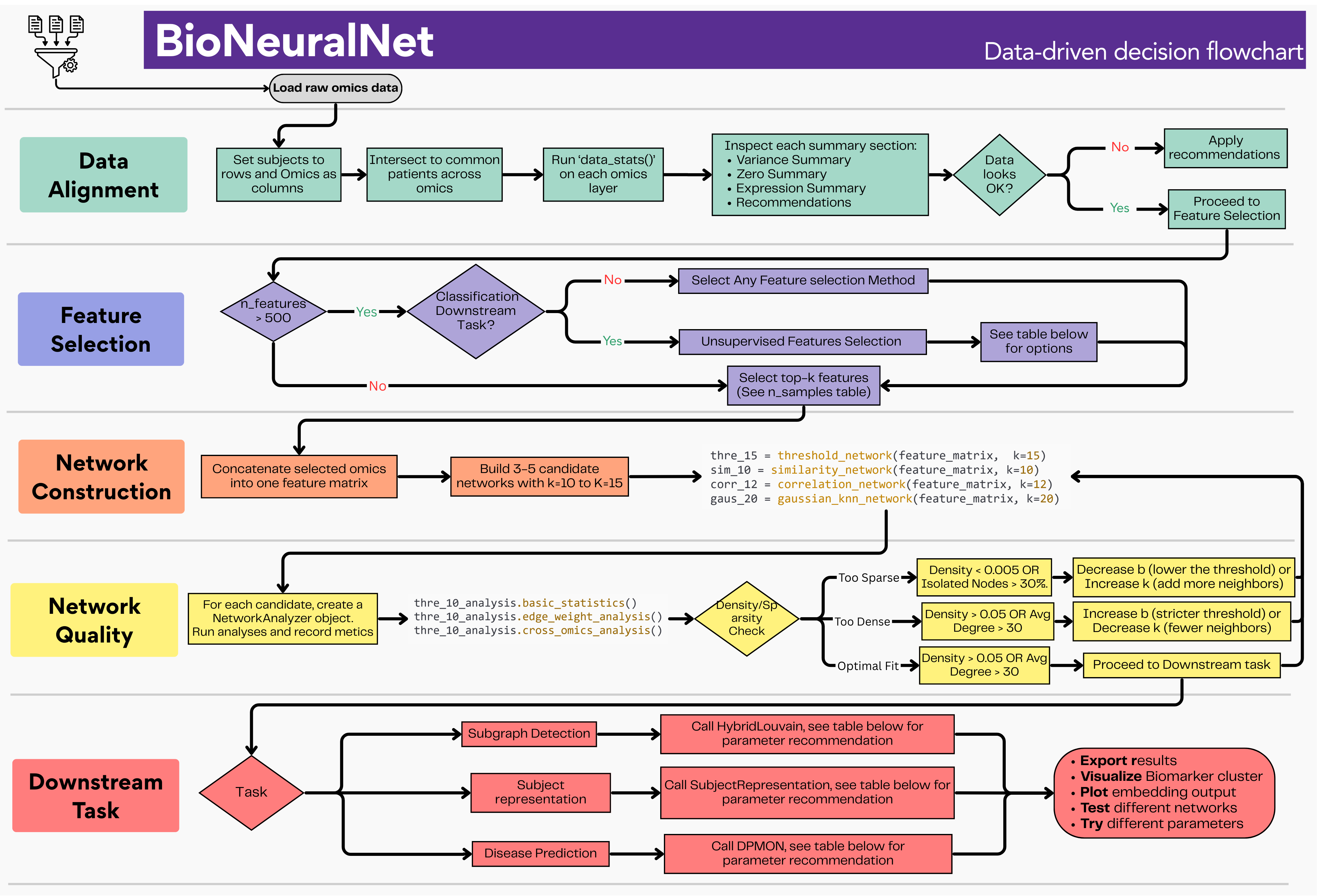
Figure: Step-by-step decision flowchart for configuring a BioNeuralNet pipeline. Details for each stage are given in the sections below. See Flow Chart Full Size
Note
For complete end-to-end code implementations on the TCGA cohorts, see the Notebooks. The BRCA, LGG, KIPAN, and ROSMAP notebooks each follow these stages from raw data alignment through downstream applications.
Stage 0: Load, Align, and Inspect Your Data
Before making any modeling decisions, standardize patient identifiers across all omics layers, align them to a common set of samples, and run a data quality assessment. This step informs every choice that follows.
0.1 - Align and standardize
import pandas as pd
from bioneuralnet.utils import m_transform, data_stats, sparse_filter

# Transpose to (samples, features) convention
mirna = mirna_raw.T
rna = rna_raw.T
meth = meth_raw.T

# Standardize patient barcodes (e.g. TCGA: keep first 12 characters)
def trim_barcode(idx):
    return idx.to_series().str.slice(0, 12)

meth.index = trim_barcode(meth.index)
rna.index = trim_barcode(rna.index)
mirna.index = trim_barcode(mirna.index)
clinical.index = clinical.index.str.upper()

# Coerce to numeric; average any duplicate rows
for df in [meth, rna, mirna]:
    df = df.apply(pd.to_numeric, errors='coerce')
    df = df.groupby(df.index).mean()

# Standardize column names
for df in [meth, rna, mirna]:
    df.columns = df.columns.str.replace(r"\?", "unknown_", regex=True)
    df.columns = df.columns.str.replace(r"\|", "_", regex=True)
    df.columns = df.columns.str.replace("-", "_", regex=False)
    df.columns = df.columns.str.replace(r"_+", "_", regex=True)
    df.columns = df.columns.str.strip("_")

# Intersect to common patients
common = sorted(set(meth.index) & set(rna.index) & set(mirna.index) & set(clinical.index))
X_meth, X_rna, X_mirna = meth.loc[common], rna.loc[common], mirna.loc[common]
Y_clinical = clinical.loc[common]
0.2 - Special case: methylation Beta values
If your methylation data consists of Beta values (bounded strictly between 0 and 1), convert them to M-values before any downstream analysis. The data_stats function will flag this automatically (see recommendation output below). M-values follow an approximately normal distribution and improve neural network stability.
# Only if data_stats flags Beta-value bounds:
X_meth = m_transform(X_meth, eps=1e-7)
0.3 - Inspect each omics layer
from bioneuralnet.utils import data_stats

data_stats(X_mirna, "miRNA")
data_stats(X_rna, "RNA")
data_stats(X_meth, "Methylation")
data_stats reports variance, sparsity, expression range, and missingness, and emits actionable recommendations. A representative output looks like:
=== miRNA Statistics Overview ===
--- Variance Summary ---
Variance Mean                   : 1.6516
Variance Median                 : 1.2756
Variance Min                    : 0.2437
Variance Max                    : 10.6028
Number Of Low Variance Features : 0

--- Zero Summary ---
Zero Mean                       : 0.0000
Number Of High Zero Features    : 0

--- Expression Summary ---
Expression Min                  : -2.7145
Expression Max                  : 18.2380

=== miRNA NaN Report ===
Global NaN: 13.72%
138 features are missing in >20.0% of samples.
54 samples are missing >20.0% of their features.

--- miRNA Recommendations ---
NORMALIZATION: Data distribution looks unbounded with low exact zeros.
Appears properly transformed.

=== Methylation Recommendations ===
NORMALIZATION: Values are strictly bounded between 0 and 1.
If these are Methylation Beta values, highly consider applying
`m_transform(df)` to convert them to M-values for neural network stability.
Decision rules from the output:
What |
Interpretation |
Action |
|---|---|---|
|
Significant missingness |
Run |
|
Degenerate features present |
Dropped automatically by |
|
Likely Beta-value methylation data |
Apply |
|
Possible raw count data (RNA-seq, miRNA) |
Consider log2 transformation |
|
Data is pre-processed; safe to proceed |
Continue to Stage 1 |
0.4 - Filter highly sparse features and samples
from bioneuralnet.utils import sparse_filter

# Drop features/samples missing in more than 20% of entries
X_mirna = sparse_filter(X_mirna, missing_fraction=0.20)
X_rna = sparse_filter(X_rna,   missing_fraction=0.20)
X_meth = sparse_filter(X_meth,  missing_fraction=0.20)

# Re-intersect after filtering (sparse_filter may drop patients)
final_patients = sorted(
  set(X_meth.index) & set(X_rna.index) &
  set(X_mirna.index) & set(Y_clinical.index)
)
X_meth, X_rna, X_mirna = (
  X_meth.loc[final_patients],
  X_rna.loc[final_patients],
  X_mirna.loc[final_patients]
)
Y_clinical = Y_clinical.loc[final_patients]

# Impute any remaining missing values with column means
for df in [X_meth, X_rna, X_mirna]:
  df.fillna(df.mean(), inplace=True)
Tip
The missing_fraction threshold of 0.20 is a reasonable starting point. For noisier data (e.g., single-cell or early-platform arrays) tighten to 0.10; for well-controlled bulk RNA-seq, 0.30 is acceptable.
Stage 1: Feature Selection
Important
Use unsupervised feature selection only prior to any train/test split. This avoids label leakage and ensures cross-validation estimates are unbiased.
Step 1.1 - Do you need feature selection?
Condition |
Recommendation |
|---|---|
n_features <= 500 |
Skip; proceed to network construction |
500 < n_features <= 5,000 |
Apply one unsupervised selector below |
n_features > 5,000 |
Feature selection is required |
Step 1.2 - How many features to keep (n_keep)?
A practical upper bound is n_samples / 2 to avoid underdetermined systems.
n_samples |
Recommended n_keep |
|---|---|
< 100 |
20 - 50 |
100 - 300 |
50 - 150 |
300 - 700 |
150 - 400 |
> 700 |
400 - 1,000 |
Step 1.3 - Which selector to use?
Selector |
Best for |
Avoid when |
Function |
|---|---|---|---|
Laplacian Score (recommended default) |
Preserving local manifold structure; heterogeneous cohorts; proven safe from leakage |
Very large feature sets (>10k) where k-NN is costly |
|
Variance Threshold |
Dense, low-dropout data; fast pre-filter |
High-sparsity data (zeros inflate variance) |
|
MAD Filter |
Skewed distributions; sparse count data; proteomics |
Gaussian-like data (variance is sufficient) |
|
PCA Loadings |
Capturing global variance directions; correlated features |
n_samples < n_features (PCA unstable) |
|
Correlation Filter (unsupervised) |
Reducing redundancy among co-expressed features |
When inter-feature correlation is expected by design |
|
Step 1.4 - Worked example
For typical high-dimensional omics (e.g., 18,000 RNA features, 511 samples):
from bioneuralnet.utils import variance_threshold, laplacian_score

# Step 1: Fast pre-filter for very high-dimensional data
X_rna_prefiltered = variance_threshold(X_rna, k=2000)

# Step 2: Laplacian Score on the reduced set
# n_keep ~ n_samples / 3; k_neighbors = 5 for dense data
X_rna_selected = laplacian_score(X_rna_prefiltered, n_keep=170, k_neighbors=5)

# For miRNA (548 features, 511 samples) - Laplacian Score directly
X_mirna_selected = laplacian_score(X_mirna, n_keep=170, k_neighbors=5)

# For methylation (20,000+ features) - two-step is required
X_meth_prefiltered = variance_threshold(X_meth, k=2000)
X_meth_selected = laplacian_score(X_meth_prefiltered, n_keep=170, k_neighbors=5)
Key parameters:
k_neighbors: use 5 for dense data; 10-15 for sparse or noisy data. Values above 20 rarely improve results.n_components(PCA Loadings only): set tomin(50, n_samples, n_features).
Stage 2: Network Construction
After feature selection, construct the multi-omics network. Build a small set of candidate networks using the same k value, inspect their topology with NetworkAnalyzer, and select the one whose density falls in the target range.
Step 2.1 - Candidate network types
Method |
Signal captured |
Typical use case |
Function |
|---|---|---|---|
Pearson correlation |
Linear co-expression |
Gene expression, proteomics |
|
Spearman correlation |
Monotonic, rank-based relationships |
Metabolomics, ordinal data |
|
Soft threshold |
Scale-free topology; strong edges emphasized |
WGCNA-style analysis |
|
Cosine similarity |
Directional similarity; magnitude-invariant |
Mixed or high-dimensional omics |
|
Gaussian k-NN |
Smooth geometric neighborhoods |
Metabolomics; continuous measurements |
|
Step 2.2 - Worked example: build and compare candidates
Start with a common k=15 and vary the construction method or power parameter.
from bioneuralnet.network import (
  correlation_network, threshold_network,
  similarity_network, gaussian_knn_network,
  NetworkAnalyzer
)
import pandas as pd

# Combine selected omics into one feature matrix
omics_combined = pd.concat([X_rna_selected, X_mirna_selected, X_meth_selected], axis=1)

# Build candidate networks
net_threshold_62 = threshold_network(omics_combined, b=6.2, k=15)
net_threshold_75 = threshold_network(omics_combined, b=7.5, k=15)
net_correlation = correlation_network(omics_combined, k=15, method='pearson')
net_similarity = similarity_network(omics_combined, k=15, metric='cosine')
net_gaussian = gaussian_knn_network(omics_combined, k=15)
Step 2.3 - Key parameters
Soft threshold (``threshold_network``)
b(power parameter): start at 6.0-6.5. Increase toward 7.5-9.0 for a sparser, more scale-free network; decrease toward 4.0 if too many edges are lost.
Correlation and similarity networks
k: start with 15. Increase if the network is too sparse after the density check.
Gaussian k-NN
k: 10-20 for typical omics. Leavesigma=Nonefor the data-adaptive estimate.
Stage 3: Network Quality Assessment
Inspect each candidate network with NetworkAnalyzer before passing it to a model. You are looking for density in the target range, no extreme hub dominance, and meaningful cross-omics edges.
Step 3.1 - Basic statistics and density check
from bioneuralnet.network import NetworkAnalyzer

analyzer = NetworkAnalyzer(net_threshold_75)
stats = analyzer.basic_statistics(threshold=0.1)
Example output:
============================================================
BASIC NETWORK STATISTICS (threshold > 0.1)
============================================================
Nodes:          430
Edges:        6,214
Density:     0.0674
Avg Degree:  28.90
Max Degree:  312
Isolated Nodes: 0 (0.0%)
Tip
These density ranges are starting points. Network behavior varies by cohort size, omics type, and construction method. Use NetworkAnalyzer diagnostics to validate before proceeding.
Measured density |
Interpretation |
Action |
|---|---|---|
> 0.7 |
Dense / Complete - noise risk high |
Increase |
0.1 - 0.7 |
Moderately dense - best performance zone |
Proceed to downstream task |
0.01 - 0.1 |
Sparse - efficient but may miss links |
Check isolated nodes; increase
|
< 0.01 |
Too sparse - network is near-empty |
Reduce |
Step 3.2 - Hub analysis
Very high-degree hub nodes can dominate GNN message passing. Check the top hubs:
hub_df = analyzer.hub_analysis(threshold=0.1, top_n=10)
If the top hub’s degree is more than 10x the average degree, raise b or reduce k to trim outlier connections.
Step 3.3 - Edge weight distribution
Use the percentile output to select a binarization threshold for topology metrics, and to understand whether the network has biologically graded signal:
weights = analyzer.edge_weight_analysis()
Total edges (weight > 0): 12,428
Mean: 0.312   Median: 0.289   Std: 0.091
Percentiles:
  25th: 0.241   50th: 0.289   75th: 0.378   90th: 0.431
Edges at different biological thresholds:
  > 0.1 : 11,904 edges
  > 0.3 :  6,214 edges
  > 0.5 :  1,832 edges
Use the 25th-50th percentile range as your threshold argument to basic_statistics and hub_analysis.
Step 3.4 - Cross-omics connectivity
For multi-omics networks, verify that between-layer interactions are present and the network is not dominated by within-layer correlations:
cross = analyzer.cross_omics_analysis(threshold=0.1)
Omics Pair           |      Edges | Max Possible |    Density
------------------------------------------------------------
rna (within)         |      4,102 |       14,535 |   0.282
mirna (within)       |        312 |       14,365 |   0.022
rna-mirna            |      1,800 |       29,070 |   0.062
A healthy multi-omics network shows cross-omics density > 0.01. If cross-omics density is near zero, the network is dominated by within-layer correlations and may not benefit from multi-omics construction. In this case, revisit feature selection or try a different construction method.
Step 3.5 - Strongest edges (sanity check)
Inspect the top interactions against known biology:
top_edges = analyzer.find_strongest_edges(top_n=10)
Step 3.6 - Selection rule
After inspecting candidates, select the network with density closest to the 0.1-0.7 range, no extreme hub dominance, and meaningful cross-omics edges. In practice, moderately dense networks have consistently yielded the best prediction accuracy [Hussein2024].
Stage 4: Downstream Task Configuration
At this point you have a cleaned feature matrix and a network in the validated density range. Configure the downstream task based on your goal.
Disease Prediction (DPMON)
The DPMON pipeline trains a GNN to generate node embeddings, reduces their dimensionality, integrates them with the raw omics features, and feeds the result to a prediction network. The entire pipeline is optimized end-to-end.
GNN Architecture
Based on systematic comparison across 15 networks in two COPD patient cohorts [Hussein2024]:
Network type |
Best architecture |
Notes |
|---|---|---|
Moderately dense |
GAT (default recommendation) |
Attention mechanism handles edge weight variation best |
Complete / Dense |
GCN or GAT (comparable) |
GCN sufficient; attention adds little at high density |
Sparse |
GAT |
Attention differentiates the few meaningful edges |
Number of GNN Layers
Network type |
Recommended layers |
Rationale |
|---|---|---|
Complete / Dense |
2 - 3 |
Over-smoothing risk is high |
Moderately dense or Sparse |
4 - 5 |
Sufficient depth to propagate information across wider neighborhoods |
Embedding Dimension
Safe range: 8 - 128. Performance gains plateau beyond 128.
Small cohorts (n < 200): stay at 8 - 32.
Large cohorts (n > 500): 64 - 128.
Dimensionality Reduction of Embeddings
Autoencoder reduction consistently yielded the strongest results across network types and densities.
Integration Method
GNN-derived scalar weights are applied via element-wise multiplication with the original omics features. This is the default and only integration method in DPMON.
Validated Reference Configurations
Validated on COPDGene multi-omics data predicting COPD GOLD stage (6 classes). Accuracy reported as mean +/- std over 500-1,000 runs [Hussein2024].
Current Smokers
Network |
GNN |
Layers |
Emb. dim |
Integration |
Accuracy |
|---|---|---|---|---|---|
1 Moderately Dense |
GAT |
4-5 |
64-128 |
Scaling |
0.5621 +/- 0.0042 |
3 Moderately Dense |
GAT |
4-5 |
64-128 |
Scaling |
0.5394 +/- 0.0009 |
1 Complete |
GCN |
2-3 |
64-128 |
Scaling |
0.5378 +/- 0.0071 |
Former Smokers
Network |
GNN |
Layers |
Emb. dim |
Integration |
Accuracy |
|---|---|---|---|---|---|
1 Moderately Dense |
GAT |
4-5 |
64-128 |
Scaling |
0.5513 +/- 0.0065 |
2 Moderately Dense |
GAT |
4-5 |
64-128 |
Scaling |
0.5491 +/- 0.0021 |
Tip
Default DPMON recipe: Moderately dense network -> GAT -> 4 layers -> embedding dim 64 -> autoencoder reduction -> scaling integration -> 2-layer prediction NN. This configuration outperforms Logistic Regression, Random Forest, SAINT, and Node2Vec by approximately 8-10%.
Subgraph Detection
For identifying biologically significant subnetworks correlated with a phenotype, the hybrid Correlated Louvain + Correlated PageRank approach [AbdelHafiz2022] is recommended over hierarchical clustering.
Correlated Louvain parameter (kL)
kL controls the balance between modularity and phenotype correlation:
kL |
Effect |
|---|---|
0.8 |
Larger subgraphs; lower correlation |
0.4-0.6 |
Balanced; default starting range |
0.0-0.2 |
Smaller, highly correlated subgraphs |
Start with kL=0.6. Use the subgraph with the highest absolute Pearson correlation to the phenotype as your result.
Correlated PageRank parameters
alpha(teleportation probability): 0.04epsilon(tolerance): 1e-6
Hybrid approach (recommended)
Run Correlated Louvain (
kL=0.6) on the full networkSelect the top subgraph by
rhoSeed Correlated PageRank weighted by node-level correlation contribution (
alpha=0.04,epsilon=1e-6)Repeat until subgraph size stabilizes
The hybrid method achieved rho = 0.41 on the COPD protein-metabolite network vs. rho = 0.33 for hierarchical clustering [AbdelHafiz2022].
Summary: Quick-Reference Recipe Table
Scenario |
Feature Selection |
Network |
GNN / Task |
Key params |
|---|---|---|---|---|
Large cohort (n>500), high-dim, disease prediction |
Variance -> Laplacian Score, n_keep=400 |
Threshold or Correlation, moderate density |
GAT, 3-4 layers, emb 64-128 |
Scaling integration, autoencoder |
Small cohort (n<200), disease prediction |
Variance or MAD, n_keep=50-100 |
Sparse to moderate; avoid complete |
GAT, 2-3 layers, emb 8-32 |
Scaling integration, 2-layer NN |
Sparse / high-dropout data (metabolomics, scRNA) |
MAD or Laplacian Score |
Gaussian k-NN |
GAT, 4-5 layers |
Impute first; inspect cross-omics density |
Subgraph / pathway detection |
Not required (operate on full network) |
Existing SmCCNet / SGTCCA network |
Hybrid Louvain + PageRank |
kL=0.6, alpha=0.04, epsilon=1e-6 |
Unknown / exploratory |
Laplacian Score, n_keep = n_samples/3 |
Pearson correlation, target density 0.1-0.7 |
GAT, 4 layers, emb 64 |
Scaling, autoencoder; tune layers first |
References
Hussein, S. et al. “Learning from Multi-Omics Networks to Enhance Disease Prediction: An Optimized Network Embedding and Fusion Approach.” In 2024 IEEE International Conference on Bioinformatics and Biomedicine (BIBM), Lisbon, Portugal, 2024, pp. 4371-4378. DOI: 10.1109/BIBM62325.2024.10822233.
Abdel-Hafiz, M., Najafi, M., et al. “Significant Subgraph Detection in Multi-omics Networks for Disease Pathway Identification.” Frontiers in Big Data, 5, 894632 (2022). DOI: 10.3389/fdata.2022.894632.