Metrics and Visualization¶

The metrics module provides a suite of tools for statistical analysis, quality control, and visualization. These functions allow users to assess data variance, explore network structures, evaluate clustering concordance, and visualize downstream performance metrics.

To see the full code used to generate the plots below (specifically for the Kidney Cancer analysis), refer to our TCGA KIPAN Biomarker Discovery tutorial in Notebooks.

Performance Evaluation¶

BioNeuralNet provides specialized plotting functions to compare model performance (e.g., Accuracy, F1-Score) across different experiments.

bioneuralnet.metrics.plot_multiple_metrics(): Visualizes multiple metrics on the same figure for comprehensive benchmarking.
bioneuralnet.metrics.plot_performance(): Plots a standard performance comparison.
bioneuralnet.metrics.plot_performance_three(): Compares three distinct metric sets side-by-side.

Example: Benchmarking GNNs vs Baselines

The following plots demonstrate a comprehensive benchmarking analysis from our TCGA KIPAN case study, comparing BioNeuralNet GNN architectures (GIN, GraphSAGE, GAT, GCN) against standard baseline models across six different performance metrics.

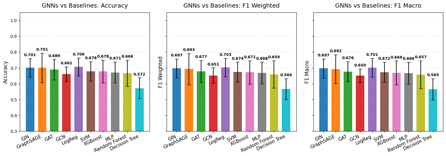
GNNs vs Baselines: Accuracy and F1 Scores

GNNs vs Baselines: Recall, AUC, and AUPR

For implementation details and parameters, refer to the API documentation: bioneuralnet.metrics.plot_multiple_metrics().

Embedding Visualization¶

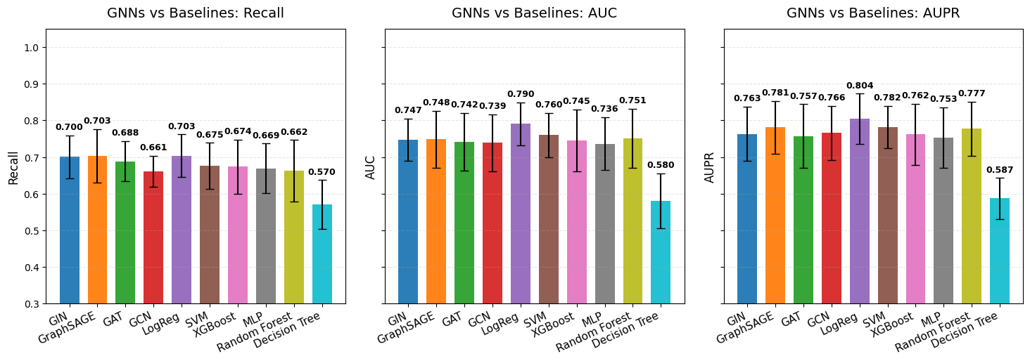
bioneuralnet.metrics.plot_embeddings() visualizes high-dimensional embeddings (e.g., from GCN or GAT models) by projecting them into a 2-dimensional space using t-SNE or UMAP.

The example below shows embeddings from the TCGA KIPAN dataset, revealing distinct clusters corresponding to different omics modalities (DNA Methylation, RNA, miRNA).

2D Projection of Embeddings from KIPAN Analysis

from bioneuralnet.metrics import plot_embeddings

# feature(omics) embeddings colored by omics type.
print(f"Plotting Feature Embeddings for graph:")
plot_embeddings(GAT_embeddings_array, node_labels, legend_labels=["DNA_Methylation", "RNA", "miRNA"])

Network Visualization & Clustering¶

These functions allow you to inspect the topology of your constructed networks and the modules identified by clustering algorithms.

Network Graph¶

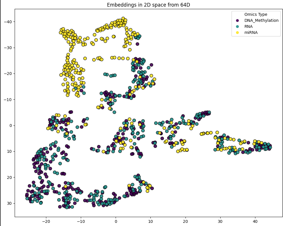
bioneuralnet.metrics.plot_network() displays the network graph from an adjacency matrix. It allows for filtering edges by weight to focus on strong connections (hubs).

Network Visualization of Hub Genes in KIPAN

from bioneuralnet.metrics import plot_network, louvain_to_adjacency

# Convert identified clusters (e.g., from Hybrid Louvain) to adjacency
louvain_adj = louvain_to_adjacency(cluster_result)

# Visualize the top connected module, filtering weak edges
plot_network(
    louvain_adj,
    weight_threshold=0.7,
    show_labels=True,
    show_edge_weights=True
)

Cluster Comparison¶

bioneuralnet.metrics.compare_clusters() allows for the visual and statistical comparison of different clustering results (e.g., comparing Hybrid Louvain results against SmCCNet results).

from bioneuralnet.metrics import compare_clusters

# Compare Hybrid Louvain results with SmCCNet clusters
compare_clusters(hybrid_result, smccnet_clusters, phenotype, merged_omics)

Correlation & Data Quality¶

These utilities help validate input data quality and quantify relationships between features and phenotypes.

Feature & Cluster Correlation¶

bioneuralnet.metrics.omics_correlation(): Computes correlation between raw omics features.
bioneuralnet.metrics.cluster_correlation(): Computes the Pearson correlation for a specific cluster of features against a phenotype.

from bioneuralnet.metrics import cluster_correlation

# Calculate correlation of a specific cluster with the phenotype
score = cluster_correlation(cluster_features, phenotype_data)

Data Variance¶

BioNeuralNet includes tools to inspect the variance within your omics datasets, which is crucial for feature selection.

bioneuralnet.metrics.plot_variance_distribution(): Plots the distribution of variances across all features.
bioneuralnet.metrics.plot_variance_by_feature(): Visualizes variance for individual features, helping to identify low-information features.

from bioneuralnet.metrics import plot_variance_distribution, plot_variance_by_feature

# Visualize the distribution of variance in the dataset
plot_variance_distribution(omics_df)

# Inspect specific feature variances to guide filtering
plot_variance_by_feature(omics_df, top_n=20)

Utilities¶

bioneuralnet.metrics.louvain_to_adjacency(): A helper function that converts the output of Louvain clustering algorithms into an adjacency matrix format suitable for plotting with plot_network.

Reference¶

For more details on each function and its parameters, see the full API reference: .. bioneuralnet.metrics API